
Nexenta Blog
Nexenta Releases Storage for Persistent Docker Containers by Storage Swiss
20 Sep 2016 by Nexenta
What if you do not consider one of the greatest advantages of containers to be an advantage to you? Many tout the stateless nature of containers as their single greatest feature. They start up, they accomplish their task, and they go away – no stateful storage necessary. Many within the container community consider a stateful container to be a violation of best practices.
And yet there is a growing desire by some to run stateful containers. One of the arguments for doing this is it allows development and production to use the exact same infrastructure. This makes it easier to move an app from development to test to production – something essential to a devops workflow. Unfortunately, however, limitations of Docker and its associated partners create difficulties for those wanting to do this….
To read more, please visit https://storageswiss.com/2016/09/20/nexenta-releases-storage-for-persistent-docker-containers/
Efficient Replication using Multicast Protocols
13 Sep 2016 by Nexenta
By Oscar Wahlberg, Director of Product Management
Replication as Data Protection
The use of replication as a data protection method is not new. Historically, it was relegated to disaster recovery for tier-1 applications and did not have a role in day-to-day backups.
Recently, however, many customers are using replication as their primary mechanism for backup and recovery for all tiers of systems – primarily due to the advent of object storage systems with built in replication and versioning. Unfortunately, the side effect is that this significantly increases the amount of data that needs to be replicated.
If one is to rely on replication as the primary method of data protection, one must replicate each version of every object to multiple nodes. Many systems transmit the entire object when it changes, then replicate the object multiple times if they are replicating it to multiple destinations. This exacerbates the issue by requiring even more bandwidth.
There is another way to protect your data…
NexentaEdge reduces the amount of bandwidth necessary to send the data to multiple nodes by doing two things: 1) using a multicast replication protocol that can send data to multiple nodes with a single transmission and 2) sending only portions that have been changed within an object instead of the entire object.
Replicast is our multicast replication protocol that allows us to transmit data to as many nodes as necessary without having to transmit it multiple times. An object is split into many chunks and each chunk transmitted by a single Replicast transmission to multiple destinations.
During transmission, the chunk is split into multiple UDP datagrams. Those destinations then reassemble received datagrams and compare them against a SHA-256 hash value for the chunk. This provides a much stronger check against data corruption than typical network checksums. Replicast transmission is intelligent enough to sustain the loss of UDP datagrams during chunk transmission and will retransmit only lost datagrams – hence, this greatly reduces bandwidth usage on busy networks.
Replicast also results in efficiencies when determining where to send data. Most replication systems decide which nodes to replicate on a round-robin basis without any consideration for how busy an individual node happens to be. Replicast uses multicast datagrams to dynamically select the storage servers for each chunk.
Instead of deciding amongst all servers, Replicast looks up a multicast group that is a subset of all nodes, then those nodes dynamically select which nodes will ultimately store the chunk. This allows fewer nodes to serve a higher number of IOPs by ensuring that the most available nodes are the ones that will receive new data, and other nodes that are congested may be given a break.
Splitting each object into chunks also gives us the ability to use cryptographic hashes to identify which chunks have changed and which haven’t. To store a new version of an object, we only need to replicate the chunks that have changed and update the metadata for that object. This results in significant bandwidth savings over alternative approaches.
Conclusion
Replication is playing a much greater role in day-to-day data protection, and there is significant room for improvement in its efficiency. The combined use of Replicast, our multicast replication protocol, and only transmitting changed chunks for new object versions is about as efficient as replication can get.
Three Dimensions of Storage Sizing & Design – Part 3: Speed
27 Jul 2016 by Nexenta
By: Edwin Weijdema
 In this third post of the multi-post Three Dimensions of Storage Sizing & Design we will dive deeper in the dimension: Use and specifically the application Workloads part characteristic Speed. Depending on the application workload requirements, you will need to size the storage system for The Need for Speed. So let us dive deeper into IOPS.
Speed with computer storage devices like hard disk drives (HDD), Solid State Drives (SSD) and Storage Area Networks (SAN) is expressed in Input/Output Per Second (IOPS). Applications will interact with storage for retrieving and storing data.
What are IOPS?
IOPS are expressing the performance a storage device can achieve with completing read and write commands in a second. We will look at a simplified example for how many IOPS a disk can deliver within the boundaries of physics. These are called the back-end IOPS. Simply put how many IOPS can the disk(s) in the back-end deliver. Every disk in your storage system has a maximum IOPS value that is based on a formula, namely:
IOPS = 1000ms / (Average Seek time in ms + Average Latency in ms)
- Rotational speed is measured in revolutions per minute (RPM). How fast the disk platters are rotating inside the disk.
- Average Latency is the time taken for the platter to undergo half a disk rotation. Why half? Well at any one time the data can be either a full disk rotation away from the head, or it might already be right at it. The time taken for a half rotation therefore gives us the average time it takes for the platter to spin round enough for the data to be retrieved. To calculate the average latency take the RPM and use the following formula: Average latency = ((60 seconds / RPM speed)/half rotation 2)*1000ms.
- Average Seek time is the time in milliseconds (ms) it takes for the disk’s head to position itself over the track being read or written. When the I/O request comes in for a particular bit of data, the head will not be above the correct track on the disk. The arm will need to move so that the head is directed over the correct track where it must then wait for the platter spin to present the target data beneath it. As the data could potentially be anywhere on the platter, the average seek time is time taken for the head to travel half way across the disk. There are both read and write seek times; by taking the average of those two values give you the average seek time.
Theoretical IOPS for Calculation Sizing
For disk (HDD and SSD) I normally use the numbers in the following table as a rule of thumb to calculate raw backend random IOPS from disks. Raw? Yes RAW, because we don’t factor in caching/buffering in the whole chain (disk, controller, head, adapter, hypervisor, operating system, application, workstation), RAID influence, interface connection, driver configurations, queue depths, etc. But lets keep this simplified to have a workable model to calculate the IOPS from the backend easily.
| Disk RPM | IOPS ~ Average | IOPS range | Average Latency (ms) |
| 5.4K HDD | 55 | 50-65 | 5,6 |
| 7.2K HDD | 80 | 75-100 | 4,2 |
| 10K HDD | 120 | 120-140 | 3,0 |
| 15K HDD | 180 | 175-210 | 2,0 |
| SSD (WI) | 40000 | 65000-115000 | 0,1** |
| SSD (MU) | 8500 | 7000-25000 | 0,1** |
| SSD (RI) | 3000 | 2000-15000 | 0,1** |
| BSSD (ICE) | 20000 | 5000-85000 | 0,1** |
** Latency on SSD is not because the spinning of the disk (duhhh no mechanical moving parts in here, latency on SSDs is on average 0.03ms!), but the network chain between the processing and the SSD. For more insight in different SSDs and their IOPS number take a look at this wiki page.
Front-End versus Back-End IOPS
Often you will hear that an application will need 2.400 IOPS and that it communicates with 64K block size. Like for instance Microsoft SQL Server 2014 OLTP Log files. These are the so-called Front-End IOPS, but to let that data land on the Back-end storage systems they generate Back-End IOPS.
Size does matter!
Lets compare a storage system that stores the data with a block size of 128K and a storage system with 4K blocks.
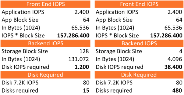
We will see that it will require 15 disks and 1.200 IOPS in the back-end when the storage system can store with 128K blocks. If you store this same I/O stream on a storage system that utilizes 4K blocks you will need a whopping 38.400 IOPS. To back those incoming IOPS you will need to run with 480x 7.2K NL-SAS disks!!!
Like most applications you can have different front-end IOPS and block sizes per workload, even within one application. Microsoft SQL 2014 server is a good example that uses a different disk access pattern as shown in the following table:
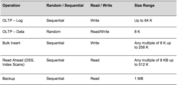
Info: Oracle DB default block size is 8K, and the Hadoop default block size is 64M.
Ok now we know that size does matter but why should you care? Most SQL Server performance issues in (virtual) environments can be traced to improper storage configuration. SQL Server workloads are generally I/O heavy, and a misconfigured storage subsystem can increase I/O latency and significantly degrade performance of SQL Server. Running Microsoft SQL server on VMware? Checkout this valuable resource about Architecting Microsoft SQL Server on VMware vSphere.
Playing the Tetris Storage Block game
With virtualization we introduce another layer into the I/O path. So what about all those different layers? If you look at a complete stack in a datacenter you could see an Application running on an Operating System that is installed within a VM. This VM runs on a Hypervisor, where this hypervisor talks to a storage backend and eventually lands on spinning disk and/or flash.
Example:
- Application – Microsoft SQL server – Logs 64K
- Operating System – Microsoft Windows 2008R2 – 4K
- Hypervisor – VMware vSphere 6 (ESXi) – runs VMFS-5 data store – 1M Unified Block
- Storage – NexentaStor 4 – 128K Block
- Disk – SanDisk BSSD – 16K block with a 4K Sector size
HDDs have a block size of 512 Bytes or 4K. With the up rise of flash we see the Block size being increased. Looking at the SanDisk – Board Solid State Drive (BSSD) card with its ICE chips gives the flash card 8TB storage capacity, which has a 16K physical block size (virtual page) and a logical 4K or 512 bytes sector size.
Block Size versus Sector Size
While sector specifically means the physical disk area, the term block has been used loosely to refer to a small chunk of data. Block has multiple meanings depending on the context. In the context of data storage, a filesystem block is an abstraction over disk sectors possibly encompassing multiple sectors. Most file systems are based on a block device, which is a level of abstraction for the hardware responsible for storing and retrieving specified blocks of data, though the block size in file systems may be a multiple of the physical block size.
Determining block size while formatting the file system in an OS is a case of tradeoffs. Every file must occupy at least one block, even if the file is zero bytes, so there’s something for the file’s metadata to be attached to. Unless you can guarantee that your files will ALWAYS be some multiple of the block size in size (e.g. in a 4k block OS, all files are 4k), there’ll be a certain amount of wastage for the files that don’t exactly fit within that block.
It’s all about Balance
Going with small block sizes is good when you need to store many small files. On the other hand, more blocks is more metadata, so you end up wasting a portion of your storage system on overhead, tracking the location of all the files. On the flip side, large blocks means less metadata, but also mean greater wastage when you’re storing small files. e.g. a 4 byte file stored in a 4k block wastes 99% of that block.
Sectors are an obsolete concept in modern drives. They existed when “locations” on a drive were specified by the old CHS (cylinder, head, sector) definition, which wasted a lot of space. All modern drives use LBA – logical block addressing, so sectors don’t really exist anymore. However, an OS can still chain multiple blocks/sector into a single logical OS-level block to reduce space. E.g. “every 8 real blocks/sectors on the drive will be considered 1 block by the Operating System”. A sector is a unit which is normally 512 bytes or 1K, 2K, 4K etc. depending on hardware.
When the logical block size of a drive is not in multiples of 512 bytes, geometry information is not available because the file system does not support other block sizes. Linux does not discover such drives, and Windows shows such drives in disk management, but does not allow you to execute any operations on them.
Partition Alignment
Aligning file system partitions is a well-known storage best practice for database workloads. Partition alignment on both physical machines and VMFS partitions prevents performance I/O degradation caused by unaligned I/O. An unaligned partition results in additional I/O operations, incurring penalty on latency and throughput. Lets look at the example we used before with the SanDisk BSSD, this BSSD uses 16KB Blocks and 4K sector sizes. For protection of the data and increasing the total amount of IOPS and throughput we stripe/mirror several cards together.
Properly Aligned
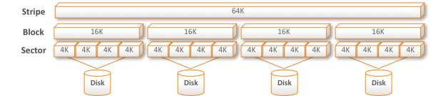
If a workload with blocksizes is properly aligned you will see that it looks like a Tetris game filling up and because of striping over more than one disk in storage systems you really want to get the most out of it.
Mis-Aligned
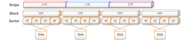
When for instance a block size of 17K is chosen for the stripe it means that you will have all kinds of problems. The Writes and Reads will cross sectors, blocks and disks carving them up into all kind of chunks and messes the data stream up with lots of additional I/O, latency and fragmentation.
Aligning with VMware vSphere 5.x or later
vSphere 5.0 and later automatically aligns VMFS-5 partitions along a 1 MB boundary (1MB Unified block). If a VMFS-3 partition was created using an earlier version of vSphere that aligned along a 64KB boundary, and that file system is then upgraded to VMFS-5, it will retain its 64KB alignment. 1 MB alignment can only be achieved when the VMFS volume is create using the vSphere Web Client.
More to the equation
There is more to the whole equation about Speed than discussed so far. Factors like:
- Protection levels like for instance RAID, where you get write penalties or multipliers with Read that effect the overall Speed. I will dive deeper and explore this further in the next blog part(s) around the Storage Dimension Protect.
- Caching on several levels in the whole I/O data path like Application, OS, Hypervisor, Host, HBA, Storage System, Disk, etc. which makes it much more complicated to predict the Speed and IOPS.
- Data reduction techniques, which I will highlight in the Storage Dimension Manage.
In the next part of Three Dimensions of Storage Sizing & Design we will dive deeper into workload characteristic Throughput (MB/s).
Raise Your SDS IQ (6 of 6): Practical Review of Containerized SDS
05 Jul 2016 by Nexenta
by Michael Letschin, Field CTO
This is the sixth of six posts (the last one was Virtual Storage Appliances) where we’re going to cover some practical details that help raise your SDS IQ and enable you to select the SDS solution that will deliver Storage on Your Terms. The sixth (and final) SDS flavor in our series is Containerized.
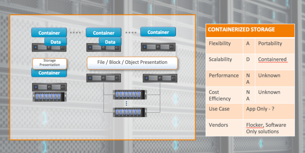
Containers are a relatively new entrant on the storage scene – and they’re hot, because unlike virtual machines, they use shared operating systems; this means they’re incredibly more efficient than hypervisors in terms of system resource usage. The big benefit is that you can get more apps (think four to six times more) on the same old servers, and you can run those apps basically anywhere. Because the container space is virtualized, storage via Containers could be considered SDS. For storage, the containerization approach varies: It’s either all local storage as in the diagram on the left, or, as on the right, external components sharing file, block, or object presentation that gets integrated into container as staple storage. You can use solutions like Flocker to get stateful storage, which is important because not every app is completely stateless.
Containerization is useful for testing in DevOps or for use in hyperscale environments; and the storage is highly portable, which means flexibility is high. Currently few enterprises are actually moving production apps into these environments, with key issues being the ability of apps to write to containers and limited (but growing) knowledge of IT staff on this new virtualization paradigm. Containers aren’t designed to scale up to accommodate a lot of storage—which enterprise apps usually need – but it may be that a solution to this emerges.. You’ll notice that we’ve let off the grades for Performance and Cost Efficiency. For Performance, because Containers run in a virtual environment, there are far too many variables to provide a standard ranking; for Cost Efficiency, again, lots of dependencies on the underlying environment, although the ability to use existing infrastructure is a big plus.
Overall grade: (soft) B – incomplete grading
See below for a typical build and the report card:
Three Dimensions of Storage Sizing & Design – Part 2: Workloads
23 Jun 2016 by Nexenta
By Edwin Weijdema, Sales Engineer, Nexenta
In this second post of the multi-post Three Dimensions of Storage Sizing & Design we will dive deeper in the dimension: Use and specifically the application Workloads part. By developing an understanding of the different kind of workloads and their characteristics will enable you to look at your different workloads and determine what impact that will have on the design and sizing. Knowing, understanding and classifying which applications will run as a workload interacting with the storage, gives you an important puzzle piece.
Knowing workloads
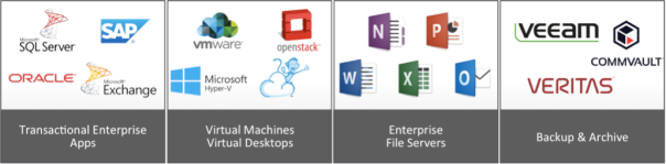
Applications have been created to support us and automate processes to work efficient and swift with the available data. Today we use, protect and manage an overwhelming amount of data that is being transformed into information through all kinds of applications. Most of these applications also interact with our storage systems. Overlooking the divers application landscape and how they interact with the storage systems(s), we can organize them in several categories where the most common ones are:
Transactional Enterprise Applications – are used to work with data that triggers an internal or external event or transaction that takes place as an organization conducts its business. A lot of people also like to simplify this by calling it the database backend. For example an online ordering system, where orders are being entered through a web interface, and than stored in a database. (e.g. SQL, Exchange, CRM, e-Business, Oracle, SAP, PostgreSQL, Sharepoint, Call Centre Systems, etc.)
Virtualization – translates the physical hardware and operating system the application runs on and creates a virtual machine in the form of a few files gathered in a folder. Most organizations are using Virtual Machines and/or Virtual Desktops to run their applications. This is a great way to consolidate infrastructures onto a few physical machines, reducing costs and making infrastructures more agile and flexible. By consolidating the different applications, servers and desktops onto a virtual environment also consolidates and changes the I/O data path to and from the storage. (e.g. VMware vSphere, VMware Horizon, Microsoft Hyper-V, Citrix Xenserver, Cloudstack, Openstack, etc.)
Generic Enterprise Fileservers – stores small to large files from all kinds of applications. Often you will see documents, pictures, media files and such. Any sort of file saved by applications and usually accessed over SMB/CIFS/NFS protocol.
Back-up & Archive – back-up and archiving systems have two distinct and complementary functions within an enterprise: backup for high-speed copy and restore to minimize the impact of failures, human error or disaster; and archiving to effectively manage data for retention and long-term access and retrieval. (e.g. Veeam, Commvault, Veritas, etc.)
Understanding workloads
Understanding workloads and specifically the Disk I/O pattern of enterprise applications helps tremendous with designing and sizing your storage solution(s). So you can make sure that your users, with their applications, are being optimal supported by the storage system. Vendors of enterprise application software often do not inform users about their workload characteristics. This is because the same application may generate different workload patterns depending upon the user’s configuration, or they simply do not know!
Workload characteristics
In this post we will just do a high level overview of the different workload characteristics and the relationship between them. In the next post we will dive deeper into the technical background of speed, throughput and response.
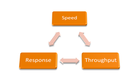
Workloads have several characteristics that define the workload type:
- Speed – measured in IOPS (Input/Output Per Second), defines the IOs per second. Read and/or Write IOs can be of different patterns (for example, sequential and random). The higher the IOPS the better the performance.
- Throughput – measured in MB/s, defines data transfer rate also often called bandwidth. The higher the throughput, the more data that can be processed per second.
- Response – measured in time like ns/us/ms latency, defines the amount of time the IO needs to complete. The lower the latency the faster a system/application/data responds, the more fluid it looks to the user. There are many latency measurements that can be taken throughout the whole data path.
Random versus Sequential access pattern
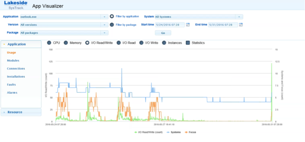
While looking at your applications and how they access their data gives you a good indication if the access pattern is random or sequential. Sequential access means all data blocks will be accessed/written after each other so 1 > 2 > 3 > 4 > 5 where Random access can mean 5 > 1 > 3 > 2 > 4. Accessing data sequentially is much faster than accessing it randomly, because of the way disk hardware works. With spinning disk the seek operation takes the most time in the whole I/O process. The disk head needs to position itself at the correct disk platter to access the requested data. Randomly reading data takes a larger number of seek operations than sequential reading, meaning that the throughput with random will be much lower than sequential. The same applies to random writing. Examining the used workloads might be useful for designing and sizing the storage system. You could use for instance Lakeside Systrack software to give a good indication in the way the workload runs and interacts with the storage.
I/O Size in the mix
The amount of throughput we can achieve is dependent on the pattern to be random or sequential and the I/O size that is being issued. For a workload with an I/O size of 4k block-size you can calculate the throughput by multiplying the number of IOPS times the I/O size.
Throughput in MB/sec = (IOPS x I/O size) / 1024
So 10.000 IOPS with an 4k block-size will be (10.000 x 4k)/1024 = 39.06 MB/sec throughput you can achieve. The whole data path should be addressed too get a clear insight and more accurate number though!
Looking at a random workload you will see that latency will start to kick in which will reduce the number of IOPS that can be achieved by the storage so random IOPS can reduce the amount of throughput significantly. A SSD produces much more IOPS and throughput against very low latency, because it does not contain moving parts. So why not go all flash than? Its all about knowing and understanding your workloads and deciphering if you need that amount of power against the cost associated with it. Balancing costs against requirements is the best way to go forward.
Classifying workloads
Lets start classifying the different workloads we identified, with the different characteristics that are important for storage. Looking at the four most common workloads:
Transactional Enterprise Applications
Transactional Enterprise Applications often are backed by a database where response is key. Looking at an Oracle database you will see that by decreasing latency will reduce the Wait states and by decreasing the Wait states the usage of CPU capacity will be reduced. If you are running virtualized Oracle database you might want to consider reducing latency and free up CPU cycles so you can run more database on that same CPU, therefore reducing your Oracle licensing cost.
Transactional Enterprise Applications tend to have a high amount of small random read I/O and a desire for fast response (low latency).
Virtualization
Virtualization is a unique workload because it consolidates several different application workloads with their corresponding characteristics on the hypervisor. So you will have several applications doing for instance random 4k, 8k and 16k blocks within the VM but the hypervisor absorbs those in memory and transforms them into 1MB or 2MB blocks which it sends and requests from the storage. VMware ESXi with VMFS5 uses 1MB unified blocks, while Microsoft Hyper-V uses 2MB blocks.
Virtualization and its consolidation also bring some storage benefit because not every application workload is going to peak at the same time. So rather than over provision it is better to look at the total picture.
Virtualization workloads tend to be fully random with a desire for speed (IOPS).
Generic Enterprise Fileserver
Generally a File Share is used by lots of users in an organization and different applications storing their data on those file shares. Users will open a file and work in/with it for some time before saving it to the file share again. So throughput to get and save the file for the user is often most important. But depending on the applications storing files it can also be that speed is required in terms of IOPS.
Generic Enterprise Fileserver workloads tend to be often sequential, but can be random with a desire for throughput (MB/s).
Back-up & Archive
Back-up & Archive workloads look like a workload that would benefit the most by maximizing throughput. This is really depending on how you use the application and which options you configure.
Lets look at for instance Veeam, the performance of many Veeam Backup & Replication functions, such as Reverse Incremental, Synthetic Full, SureBackup and Instant Restore are most impact by the ability of the storage array to deliver random IOPS.
Veeam Backup & Replication offers two primary modes for storing backups to disk, Forward and Reverse incremental. Due to the differences in how these modes write backups to disk they have very different storage I/O profiles.
Forward Incremental backups offer the advantage that they perform only sequential writes to the target repository meaning that performance is significantly higher than reverse incremental backups. However, this backup mode does come with costs, primarily in the requirement to schedule periodic full backups. These backups will take additional time to create and, based on the method, addition space on the target repository.
There are three options for creating new full backups:
Synthetic Full — this method uses the most recent full backup, and any incremental backups created since then and builds a new full backup using this data. This requires space for a new full backup, and random I/O on the target repository and can take a long time to process.
Synthetic Full w/Transform — this method uses the most recent full backup, and any incremental backups created since then and builds a new full backup using this data, while converting the incremental backups to reverse incremental files. This requires only a small amount of additional space on the target repository, but usage a large amount of random I/O and can take a very long time to process
Active Full — this method simply runs a new full backup by reading all data from the source VMs. This requires I/O on the source storage, enough space to store a new full backup and sequential write I/O on the target repository.
Back-up & Archive workloads tend to be often sequential, but can be fully random with a high desire for throughput (MB/s) and speed (IOPS).
Summary
Interestingly, workload characterization is not only useful for sizing and designing storage systems but also useful for application developers to help them optimize their I/O routines or to document best practices based on such analysis. In the next part of Three Dimensions of Storage Sizing & Design we will dive deeper into workload characteristics speed (IOPS), throughput (MB/s) and Response (ms).